Welcome to the ultimate guide on Data Acquisition (DAQ) systems! Whether you're an engineer, scientist, student, or hobbyist, this resource will take you from fundamental concepts to advanced implementations. DAQ systems are the backbone of modern measurement and control applications, enabling us to capture real-world phenomena and transform them into actionable digital data.
1. What is Data Acquisition (DAQ)?
Data Acquisition (DAQ) is the process of sampling signals that measure real-world physical conditions and converting the resulting samples into digital numeric values that can be manipulated by a computer. DAQ systems typically consist of sensors, signal conditioning hardware, analog-to-digital converters (ADCs), and software for data processing and analysis.
At its core, DAQ bridges the gap between the analog world we live in and the digital world of computers. Without DAQ systems, we wouldn't be able to monitor temperature in industrial processes, record neural activity in neuroscience research, or test structural integrity in aerospace engineering.
# Basic DAQ workflow concept
import numpy as np

# Simulate analog signal from sensor
time = np.linspace(0, 10, 1000)  # 10 seconds, 1000 samples
analog_signal = np.sin(2 * np.pi * time) + 0.1 * np.random.randn(len(time))

# Simulate ADC conversion (quantization)
digital_signal = np.round(analog_signal * 100) / 100  # 2 decimal precision

print(f"Original signal range: [{analog_signal.min():.2f}, {analog_signal.max():.2f}]")
print(f"Digitized signal range: [{digital_signal.min():.2f}, {digital_signal.max():.2f}]")
2. Why Data Acquisition Matters in Modern Technology
DAQ systems are critical because they enable us to make informed decisions based on real-world data. In manufacturing, DAQ systems monitor production lines to ensure quality control. In healthcare, they capture vital signs for patient monitoring. In environmental science, they track climate changes through sensor networks. The importance of DAQ cannot be overstated—it's the foundation of the Internet of Things (IoT), Industry 4.0, and smart infrastructure.
Without reliable DAQ systems, we'd be operating blindly in complex systems. Imagine trying to optimize a chemical reaction without knowing the temperature, or flying an aircraft without airspeed indicators. DAQ provides the eyes and ears for our technological systems.
# Simulate industrial temperature monitoring
import time
import random

def read_temperature_sensor():
    """Simulate reading from a temperature sensor"""
    base_temp = 25.0  # Room temperature
    fluctuation = random.uniform(-2.0, 2.0)
    noise = random.uniform(-0.5, 0.5)
    return base_temp + fluctuation + noise

# Continuous monitoring loop
for minute in range(10):
    temp = read_temperature_sensor()
    timestamp = time.strftime("%Y-%m-%d %H:%M:%S")
    print(f"[{timestamp}] Temperature: {temp:.2f}°C")

    # Alert if temperature exceeds threshold
    if temp > 28.0:
        print("   *** ALERT: Temperature above safe threshold! ***")

    time.sleep(1)  # Simulate 1-second intervals
3. Core Components of a DAQ System
Every DAQ system consists of several key components working together: sensors (transducers that convert physical phenomena into electrical signals), signal conditioning circuitry (amplifiers, filters, isolators), analog-to-digital converters (ADCs), data storage/processing units, and software interfaces. Understanding each component is essential for designing effective DAQ solutions.
Sensors are the "front line" of any DAQ system—they directly interact with the physical parameter being measured. Signal conditioning prepares the sensor output for digitization by amplifying weak signals, filtering noise, or converting signal types. The ADC is the heart of the system, determining resolution, sampling rate, and accuracy.
class DAQSystem:
    def __init__(self, sensor_type, sampling_rate, resolution_bits):
        self.sensor_type = sensor_type
        self.sampling_rate = sampling_rate  # samples per second
        self.resolution = 2**resolution_bits  # number of discrete levels
        self.data_buffer = []

    def read_sensor(self):
        """Simulate reading from a sensor"""
        if self.sensor_type == "temperature":
            return random.uniform(20.0, 30.0)
        elif self.sensor_type == "pressure":
            return random.uniform(950.0, 1050.0)
        else:
            return random.uniform(0, 10)

    def digitize(self, analog_value, range_min=0, range_max=10):
        """Convert analog value to digital based on resolution"""
        normalized = (analog_value - range_min) / (range_max - range_min)
        digital_value = int(normalized * (self.resolution - 1))
        return digital_value

    def acquire_sample(self):
        """Acquire and digitize one sample"""
        analog = self.read_sensor()
        digital = self.digitize(analog)
        self.data_buffer.append(digital)
        return analog, digital

# Create a temperature DAQ system
daq = DAQSystem("temperature", sampling_rate=100, resolution_bits=12)
analog_val, digital_val = daq.acquire_sample()
print(f"Analog: {analog_val:.2f} -> Digital: {digital_val} (12-bit)")
4. Analog-to-Digital Conversion Fundamentals
Analog-to-Digital Conversion (ADC) is the process of converting continuous analog signals into discrete digital representations. Key ADC characteristics include resolution (number of bits), sampling rate (samples per second), and accuracy. The Nyquist-Shannon sampling theorem states that to accurately reconstruct a signal, the sampling rate must be at least twice the highest frequency component in the signal.
Understanding ADC limitations is crucial—aliasing occurs when signals are undersampled, quantization error is inherent in the digitization process, and noise can corrupt measurements. High-resolution ADCs (16-bit, 24-bit) are essential for precision applications like scientific instrumentation.
import numpy as np
import matplotlib.pyplot as plt

# Create a high-frequency signal
fs_original = 1000  # Original sampling rate (Hz)
t = np.linspace(0, 1, fs_original)
high_freq_signal = np.sin(2 * np.pi * 200 * t)  # 200 Hz signal

# Undersample the signal (violating Nyquist)
fs_undersampled = 300  # Below Nyquist rate (should be >400 Hz)
t_undersampled = np.linspace(0, 1, fs_undersampled)
undersampled_signal = np.sin(2 * np.pi * 200 * t_undersampled)

# Calculate aliased frequency
aliased_freq = abs(200 - fs_undersampled)  # 100 Hz alias

print(f"Original frequency: 200 Hz")
print(f"Sampling rate: {fs_undersampled} Hz (Nyquist rate: 400 Hz)")
print(f"Aliased frequency: {aliased_freq} Hz")

# Plot would show the aliasing effect (not rendered here)
5. Signal Conditioning Techniques
Signal conditioning prepares sensor outputs for accurate digitization. Common techniques include amplification (boosting weak signals), filtering (removing noise outside the frequency band of interest), isolation (protecting equipment from high voltages), and linearization (correcting nonlinear sensor responses). Proper signal conditioning can dramatically improve measurement accuracy and system reliability.
For example, thermocouple signals are typically in the millivolt range and require amplification before ADC conversion. Strain gauges often need Wheatstone bridge circuits and instrumentation amplifiers. Understanding the electrical characteristics of your sensors is essential for effective signal conditioning design.
import numpy as np

def apply_signal_conditioning(raw_signal, gain=10, cutoff_freq=10, fs=1000):
    """
    Simulate basic signal conditioning:
    - Amplification (gain)
    - Low-pass filtering (removes high-frequency noise)
    """
    # Amplify the signal
    amplified = raw_signal * gain

    # Simple low-pass filter (moving average)
    window_size = int(fs / cutoff_freq)
    filtered = np.convolve(amplified, np.ones(window_size)/window_size, mode='same')

    return filtered

# Simulate noisy sensor signal
time = np.linspace(0, 5, 5000)
true_signal = 0.1 * np.sin(2 * np.pi * 2 * time)  # 2 Hz signal
noise = 0.05 * np.random.randn(len(time))
raw_sensor = true_signal + noise

# Apply conditioning
conditioned = apply_signal_conditioning(raw_sensor, gain=20, cutoff_freq=5)

print(f"Raw signal SNR: {np.var(true_signal)/np.var(noise):.2f}")
print(f"Conditioned signal shows improved clarity")
6. Choosing the Right Sensors for Your Application
Selecting appropriate sensors is critical for successful DAQ implementation. Considerations include measurement range, accuracy, response time, environmental conditions, power requirements, and output signal type. Common sensor types include thermocouples (temperature), strain gauges (force/pressure), accelerometers (vibration), and photodiodes (light).
For instance, in a high-temperature industrial environment, you might choose a Type K thermocouple over an RTD due to its wider temperature range. In precision medical applications, you might select a platinum RTD for its excellent stability and accuracy. Always match sensor specifications to your application requirements.
class Sensor:
    def __init__(self, name, measurement_type, range_min, range_max, accuracy, cost):
        self.name = name
        self.type = measurement_type
        self.range_min = range_min
        self.range_max = range_max
        self.accuracy = accuracy
        self.cost = cost

    def is_suitable(self, required_min, required_max, max_cost):
        """Check if sensor meets requirements"""
        in_range = (self.range_min <= required_min and
                   self.range_max >= required_max)
        affordable = self.cost <= max_cost
        return in_range and affordable

# Define available sensors
sensors = [
    Sensor("Thermocouple K", "Temperature", -200, 1260, 2.2, 25),
    Sensor("PT100 RTD", "Temperature", -200, 600, 0.3, 85),
    Sensor("DS18B20", "Temperature", -55, 125, 0.5, 5)
]

# Application requirements
required_temp_min = -50
required_temp_max = 100
budget = 50

# Find suitable sensors
suitable = [s for s in sensors if s.is_suitable(required_temp_min, required_temp_max, budget)]
for sensor in suitable:
    print(f"Recommended: {sensor.name} (Accuracy: ±{sensor.accuracy}°C, Cost: ${sensor.cost})")
7. Sampling Rate and Nyquist Theorem
The Nyquist-Shannon sampling theorem is fundamental to DAQ: to accurately reconstruct a signal, you must sample at least twice the highest frequency component present. This minimum rate is called the Nyquist rate. In practice, engineers often sample at 5-10 times the highest frequency to ensure accurate representation and account for filter roll-off.
Undersampling leads to aliasing—where high-frequency components appear as lower frequencies in the digitized signal. Anti-aliasing filters (low-pass filters) are essential before ADC to remove frequencies above the Nyquist frequency. Understanding your signal's frequency content through spectral analysis is crucial for proper sampling rate selection.
def calculate_nyquist_rate(max_frequency, safety_factor=5):
    """
    Calculate appropriate sampling rate based on Nyquist theorem
    with safety factor for real-world applications
    """
    nyquist_rate = 2 * max_frequency
    practical_rate = safety_factor * max_frequency
    return nyquist_rate, practical_rate

# Example: Audio signal with 20 kHz maximum frequency
max_freq = 20000  # 20 kHz
nyquist, practical = calculate_nyquist_rate(max_freq)

print(f"Signal maximum frequency: {max_freq/1000:.1f} kHz")
print(f"Absolute minimum (Nyquist): {nyquist/1000:.1f} kHz")
print(f"Recommended sampling rate: {practical/1000:.1f} kHz")
print(f"Standard audio CD rate: 44.1 kHz")
8. Resolution and Quantization Error
ADC resolution determines how finely an analog signal can be divided into discrete levels. An N-bit ADC has 2^N possible output values. Quantization error is the difference between the actual analog value and the nearest digital representation—it's an inherent limitation of digitization. Higher resolution reduces quantization error but increases cost and data volume.
For example, a 12-bit ADC measuring 0-10V has a resolution of 10V/4096 ≈ 2.44mV per step. A 16-bit ADC on the same range has 10V/65536 ≈ 0.15mV resolution—16 times finer. Choose resolution based on your required measurement precision and signal-to-noise ratio.
def calculate_quantization_error(voltage_range, bits):
    """Calculate quantization error for given ADC specs"""
    steps = 2 ** bits
    step_size = voltage_range / steps
    max_error = step_size / 2  # Maximum quantization error
    return step_size, max_error

# Compare different ADC resolutions
voltage_range = 10.0  # 0-10V range

for bits in [8, 12, 16, 24]:
    step, error = calculate_quantization_error(voltage_range, bits)
    print(f"{bits}-bit ADC: Step size = {step*1000:.3f} mV, Max error = ±{error*1000:.3f} mV")

# Practical implication
measured_voltage = 3.14159
for bits in [12, 16]:
    step, _ = calculate_quantization_error(voltage_range, bits)
    digitized = round(measured_voltage / step) * step
    error = abs(measured_voltage - digitized)
    print(f"{bits}-bit representation of {measured_voltage}V: {digitized:.6f}V (error: {error*1000:.3f} mV)")
9. DAQ Hardware Interfaces: USB, Ethernet, PCIe
Modern DAQ systems connect to computers through various interfaces, each with trade-offs in speed, distance, and complexity. USB offers plug-and-play convenience for portable applications. Ethernet enables long-distance connections and network integration. PCIe provides the highest bandwidth for demanding applications like high-speed imaging or RF analysis.
When selecting an interface, consider data throughput requirements, cable length needs, and synchronization capabilities. USB 3.0 can handle up to 5 Gbps, Gigabit Ethernet provides 1 Gbps over 100m, while PCIe x16 offers over 15 GB/s. For distributed systems, Ethernet-based DAQ (like LXI standard) is often preferred.
interfaces = {
    "USB 2.0": {"speed_mbps": 480, "max_distance_m": 5},
    "USB 3.0": {"speed_mbps": 5000, "max_distance_m": 3},
    "Gigabit Ethernet": {"speed_mbps": 1000, "max_distance_m": 100},
    "PCIe x1": {"speed_mbps": 1000, "max_distance_m": 0.5},  # On motherboard
    "PCIe x16": {"speed_mbps": 16000, "max_distance_m": 0.5}
}

# Calculate maximum channels for 16-bit, 100 kS/s per channel
sample_rate_per_channel = 100000  # 100 kS/s
bits_per_sample = 16
bytes_per_sample = bits_per_sample / 8

print("Max channels for 100 kS/s, 16-bit sampling:")
for name, specs in interfaces.items():
    max_channels = specs["speed_mbps"] * 1e6 / (sample_rate_per_channel * bytes_per_sample * 8)
    print(f"{name:20}: {max_channels:6.0f} channels (max distance: {specs['max_distance_m']}m)")
10. Synchronization in Multi-Channel DAQ
When acquiring data from multiple channels simultaneously, synchronization ensures all measurements are time-aligned. This is critical for applications like vibration analysis (where phase relationships matter) or power quality monitoring (where voltage and current must be measured at the exact same instant). DAQ systems use various synchronization methods including shared clocks, trigger signals, and time-stamping.
Hardware synchronization (using dedicated sync lines) provides the highest precision, while software synchronization is simpler but less accurate. For distributed systems, protocols like IEEE 1588 Precision Time Protocol (PTP) can synchronize devices across networks to sub-microsecond accuracy.
import time
import threading

class SynchronizedDAQ:
    def __init__(self, num_channels):
        self.num_channels = num_channels
        self.data = [[] for _ in range(num_channels)]
        self.sync_event = threading.Event()

    def read_channel(self, channel_id):
        """Simulate reading from a channel with synchronization"""
        self.sync_event.wait()  # Wait for synchronization signal
        start_time = time.time()

        # Simulate acquisition
        for i in range(100):
            # Simulate sensor reading with channel-specific characteristics
            value = 0.5 * channel_id + 0.1 * i + 0.01 * (time.time() - start_time)
            self.data[channel_id].append(value)
            time.sleep(0.001)  # 1ms per sample

    def acquire_synchronized(self):
        """Start synchronized acquisition across all channels"""
        threads = []
        self.sync_event.clear()

        # Start all channel threads
        for ch in range(self.num_channels):
            t = threading.Thread(target=self.read_channel, args=(ch,))
            t.start()
            threads.append(t)

        # Trigger synchronization after brief delay
        time.sleep(0.01)
        self.sync_event.set()

        # Wait for all threads to complete
        for t in threads:
            t.join()

# Example usage
daq = SynchronizedDAQ(4)
daq.acquire_synchronized()
print(f"Acquired {len(daq.data[0])} samples per channel with synchronization")
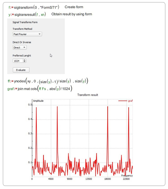
11. Real-Time Data Processing Techniques
Real-time processing analyzes data as it's acquired, enabling immediate feedback and control. Techniques include digital filtering, Fast Fourier Transforms (FFT) for frequency analysis, peak detection, and statistical calculations. Real-time processing requires careful resource management to ensure processing completes before the next data arrives.
For high-speed applications, consider using optimized libraries (like NumPy), compiled code (C/C++ extensions), or specialized hardware (FPGAs). Buffer management is critical—circular buffers prevent data loss during processing. Always profile your processing pipeline to ensure it meets timing requirements.
class RealTimeMovingAverage:
    def __init__(self, window_size):
        self.window_size = window_size
        self.buffer = []
        self.sum = 0

    def update(self, new_value):
        """Add new value and return filtered output"""
        self.buffer.append(new_value)
        self.sum += new_value

        if len(self.buffer) > self.window_size:
            removed = self.buffer.pop(0)
            self.sum -= removed

        return self.sum / len(self.buffer)

# Simulate real-time processing
import random
filter = RealTimeMovingAverage(window_size=10)
raw_data = [random.uniform(0, 10) for _ in range(100)]
filtered_data = [filter.update(x) for x in raw_data]

print(f"First 5 raw values: {[f'{x:.2f}' for x in raw_data[:5]]}")
print(f"First 5 filtered values: {[f'{x:.2f}' for x in filtered_data[:5]]}")
12. Data Storage and Management Strategies
Efficient data storage is crucial for DAQ systems, especially those running long-term experiments. Considerations include file formats (binary vs. text), compression, metadata inclusion, and database integration. HDF5 is popular for scientific data due to its hierarchical structure and compression capabilities. For high-speed applications, binary formats minimize I/O overhead.
Always include metadata with your data—sampling rate, sensor calibration, units, and timestamps are essential for later analysis. For large-scale deployments, consider database solutions like InfluxDB (time-series optimized) or traditional SQL databases with appropriate indexing.
# Requires: pip install h5py numpy
import h5py
import numpy as np
import time

def save_daq_data_to_hdf5(filename, data, sampling_rate, sensor_info):
    """Save DAQ data with metadata to HDF5 file"""
    with h5py.File(filename, 'w') as f:
        # Create dataset
        dset = f.create_dataset('data', data=data, compression='gzip')

        # Add metadata as attributes
        dset.attrs['sampling_rate'] = sampling_rate
        dset.attrs['timestamp'] = time.time()
        dset.attrs['units'] = 'volts'
        dset.attrs['sensor_type'] = sensor_info['type']
        dset.attrs['calibration_date'] = sensor_info['calibration_date']

        print(f"Data saved to {filename} with metadata")

# Example usage
simulated_data = np.random.randn(10000).astype(np.float32)
sensor_metadata = {
    'type': 'accelerometer',
    'calibration_date': '2023-01-15'
}

save_daq_data_to_hdf5('experiment_001.h5', simulated_data, 1000, sensor_metadata)
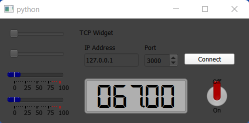
13. Building a Python-Based DAQ GUI
Creating a graphical user interface (GUI) for your DAQ system makes it accessible to non-programmers and provides real-time visualization. Python libraries like PyQt5/6, Tkinter, or matplotlib's animation capabilities are excellent choices. A well-designed DAQ GUI should include controls for configuration, real-time plots, data logging options, and alarm indicators.
When designing your GUI, prioritize responsiveness—use threading to prevent the interface from freezing during data acquisition. Implement proper error handling for hardware communication failures. Consider user experience: intuitive controls, clear visual feedback, and consistent layout improve usability significantly.
# Requires: pip install matplotlib numpy
import matplotlib.pyplot as plt
import matplotlib.animation as animation
import numpy as np
import random

class SimpleDAQGUI:
    def __init__(self, max_points=100):
        self.max_points = max_points
        self.x_data = list(range(max_points))
        self.y_data = [0] * max_points

        # Setup plot
        self.fig, self.ax = plt.subplots()
        self.line, = self.ax.plot(self.x_data, self.y_data)
        self.ax.set_ylim(-2, 2)
        self.ax.set_title('Real-time DAQ Visualization')
        self.ax.set_xlabel('Time (samples)')
        self.ax.set_ylabel('Amplitude')

    def update(self, frame):
        """Update plot with new data point"""
        # Simulate reading from DAQ hardware
        new_value = np.sin(frame/10) + 0.1*random.random()

        # Update data buffer
        self.y_data = self.y_data[1:] + [new_value]
        self.line.set_ydata(self.y_data)
        return self.line,

    def start(self):
        """Start the animation"""
        ani = animation.FuncAnimation(
            self.fig, self.update, interval=50, blit=True
        )
        plt.show()

# Uncomment to run:
# gui = SimpleDAQGUI()
# gui.start()
14. Error Handling and System Reliability
Robust DAQ systems must handle various error conditions gracefully: sensor disconnections, communication timeouts, buffer overflows, and hardware failures. Implement comprehensive error handling with try-except blocks, timeouts for hardware operations, and data validation checks. Logging errors with timestamps helps diagnose intermittent issues.
For critical applications, consider redundancy—dual sensors, backup communication paths, or fail-safe modes. Always validate incoming data against expected ranges; a temperature reading of 10,000°C likely indicates a sensor fault rather than a real measurement. Graceful degradation (continuing with reduced functionality) is better than complete system failure.
import time
import logging

logging.basicConfig(level=logging.INFO)
logger = logging.getLogger('DAQ_System')

class RobustDAQ:
    def __init__(self, sensor_id):
        self.sensor_id = sensor_id
        self.connected = False
        self.last_reading = None

    def connect(self):
        """Simulate hardware connection with error handling"""
        try:
            # Simulate connection attempt
            if random.random() > 0.1:  # 90% success rate
                self.connected = True
                logger.info(f"Sensor {self.sensor_id} connected successfully")
            else:
                raise ConnectionError("Hardware communication timeout")
        except Exception as e:
            logger.error(f"Connection failed for sensor {self.sensor_id}: {str(e)}")
            self.connected = False

    def read_safe(self, timeout=2.0):
        """Read with timeout and validation"""
        if not self.connected:
            self.connect()
            if not self.connected:
                return None

        start_time = time.time()
        try:
            # Simulate reading with possible timeout
            time.sleep(0.1)  # Simulate read time
            if time.time() - start_time > timeout:
                raise TimeoutError("Sensor read timeout")

            # Simulate reading
            raw_value = random.uniform(-10, 10)

            # Validate reading
            if not (-5 <= raw_value <= 5):
                logger.warning(f"Out-of-range reading from {self.sensor_id}: {raw_value}")
                return None

            self.last_reading = raw_value
            return raw_value

        except Exception as e:
            logger.error(f"Read error for {self.sensor_id}: {str(e)}")
            return None

# Example usage
daq = RobustDAQ("TEMP-01")
for i in range(5):
    value = daq.read_safe()
    if value is not None:
        print(f"Valid reading: {value:.2f}")
    else:
        print("Invalid reading - using last known good value")
15. Calibration and Accuracy Verification
Calibration ensures your DAQ system provides accurate measurements by comparing readings against known standards. Regular calibration accounts for sensor drift, amplifier gain changes, and ADC nonlinearities. Calibration procedures typically involve measuring known reference values (e.g., ice bath for 0°C, precision voltage sources) and creating correction curves.
Accuracy verification should be part of your system validation process. Document calibration dates, procedures, and results. For critical applications, implement automated calibration routines that run during system startup. Remember that calibration is only valid for the conditions under which it was performed—temperature, humidity, and other environmental factors can affect accuracy.
import numpy as np
from scipy.interpolate import interp1d

class CalibratedSensor:
    def __init__(self, raw_readings, true_values):
        """
        Create calibration from reference measurements
        raw_readings: list of raw sensor outputs
        true_values: corresponding known true values
        """
        # Create interpolation function for calibration
        self.calibration_curve = interp1d(
            raw_readings, true_values,
            kind='linear', fill_value='extrapolate'
        )

    def read_calibrated(self, raw_value):
        """Convert raw reading to calibrated value"""
        return float(self.calibration_curve(raw_value))

# Example: Temperature sensor calibration
raw_temps = [0.1, 0.5, 1.0, 1.5, 2.0]  # Raw sensor outputs (V)
true_temps = [0, 25, 50, 75, 100]       # Known temperatures (°C)

calibrated_sensor = CalibratedSensor(raw_temps, true_temps)

# Test with new readings
test_readings = [0.3, 0.8, 1.7]
for raw in test_readings:
    calibrated = calibrated_sensor.read_calibrated(raw)
    print(f"Raw: {raw}V -> Calibrated: {calibrated:.1f}°C")
16. Advanced Triggering and Event Detection
Advanced triggering allows DAQ systems to capture data only when specific conditions occur, saving storage and processing resources. Trigger types include level triggers (when signal crosses threshold), edge triggers (on rising/falling edges), window triggers (when signal enters/leaves range), and pattern triggers (for digital inputs).
Event detection goes beyond simple triggering—it identifies complex patterns like peaks, zero-crossings, or specific waveforms. Implementing these in software requires careful algorithm design to avoid missing events or generating false positives. Hardware triggers provide the lowest latency and highest reliability for critical applications.
class AdvancedTrigger:
    def __init__(self, trigger_type, threshold=None, window=None):
        self.trigger_type = trigger_type
        self.threshold = threshold
        self.window = window
        self.last_state = False

    def check_trigger(self, current_value):
        """Check if trigger condition is met"""
        triggered = False

        if self.trigger_type == "level_rising":
            if current_value >= self.threshold and not self.last_state:
                triggered = True
        elif self.trigger_type == "window_entry":
            if self.window[0] <= current_value <= self.window[1]:
                triggered = True
        elif self.trigger_type == "peak":
            # Simplified peak detection (requires history)
            pass

        self.last_state = current_value >= self.threshold
        return triggered

# Example usage
trigger = AdvancedTrigger("level_rising", threshold=2.5)
test_values = [1.0, 2.0, 2.4, 2.6, 3.0, 2.8]

for i, value in enumerate(test_values):
    if trigger.check_trigger(value):
        print(f"Trigger activated at sample {i} with value {value}")
17. Distributed DAQ Systems Architecture
Distributed DAQ systems deploy multiple acquisition nodes across a physical area, connected via network protocols. This architecture is essential for large-scale applications like structural health monitoring of bridges, environmental sensor networks, or factory-wide process control. Key challenges include synchronization, data aggregation, and network reliability.
Modern distributed DAQ often uses IoT protocols (MQTT, CoAP) for efficient communication. Edge computing nodes can preprocess data locally before transmission, reducing bandwidth requirements. Time synchronization across nodes is critical—consider GPS timing or IEEE 1588 PTP for sub-millisecond accuracy across large installations.
import json
import time
import uuid

class DAQNode:
    def __init__(self, node_id, location):
        self.node_id = node_id
        self.location = location
        self.sensors = {}

    def add_sensor(self, sensor_id, sensor_type):
        self.sensors[sensor_id] = {
            'type': sensor_type,
            'last_reading': None,
            'last_update': None
        }

    def read_sensors(self):
        """Read all sensors and return data packet"""
        data_packet = {
            'node_id': self.node_id,
            'location': self.location,
            'timestamp': time.time(),
            'readings': {}
        }

        for sensor_id in self.sensors:
            # Simulate sensor reading
            if self.sensors[sensor_id]['type'] == 'temperature':
                value = 20 + 5 * (hash(sensor_id) % 10) / 10
            else:
                value = random.uniform(0, 100)

            data_packet['readings'][sensor_id] = {
                'value': value,
                'unit': 'C' if self.sensors[sensor_id]['type'] == 'temperature' else 'units'
            }

        return data_packet

# Create distributed system
nodes = [
    DAQNode("NODE-01", "Building A, Floor 1"),
    DAQNode("NODE-02", "Building A, Floor 2"),
    DAQNode("NODE-03", "Building B, Ground Floor")
]

for node in nodes:
    node.add_sensor(f"TEMP-{node.node_id}", "temperature")
    node.add_sensor(f"HUMID-{node.node_id}", "humidity")

# Simulate data collection
for node in nodes:
    packet = node.read_sensors()
    print(f"Data from {packet['location']}: {len(packet['readings'])} sensors")
18. Security Considerations for Networked DAQ
As DAQ systems become increasingly connected, security is paramount. Networked DAQ devices can be entry points for cyber attacks, potentially compromising entire industrial control systems. Implement security best practices: strong authentication, encrypted communications (TLS/SSL), regular firmware updates, and network segmentation.
For critical infrastructure, consider air-gapped systems or unidirectional gateways that prevent remote access while allowing data export. Always change default passwords, disable unused services, and implement role-based access control. Security should be designed in from the beginning—not added as an afterthought.
import ssl
import socket
import hashlib

class SecureDAQClient:
    def __init__(self, server_host, server_port, cert_file):
        self.server_host = server_host
        self.server_port = server_port
        self.cert_file = cert_file

    def connect_securely(self):
        """Establish secure TLS connection to DAQ server"""
        context = ssl.create_default_context(ssl.Purpose.SERVER_AUTH)
        context.load_verify_locations(self.cert_file)

        # Create socket and wrap with TLS
        sock = socket.socket(socket.AF_INET, socket.SOCK_STREAM)
        secure_sock = context.wrap_socket(sock, server_hostname=self.server_host)

        try:
            secure_sock.connect((self.server_host, self.server_port))
            print("Secure connection established")
            return secure_sock
        except Exception as e:
            print(f"Connection failed: {e}")
            return None

    def send_authenticated_data(self, data, secret_key):
        """Send data with HMAC authentication"""
        # Create message authentication code
        mac = hashlib.sha256((data + secret_key).encode()).hexdigest()
        secure_message = f"{data}|{mac}"

        # In real implementation, send over secure_sock
        print(f"Sending authenticated data: {secure_message[:50]}...")

# Example usage (requires proper certificates)
# client = SecureDAQClient("daq-server.example.com", 8443, "server-cert.pem")
# secure_socket = client.connect_securely()
# if secure_socket:
#     client.send_authenticated_data("sensor_data=23.5", "my_secret_key")
19. Performance Optimization for High-Speed DAQ
High-speed DAQ applications (MHz sampling rates) demand careful performance optimization. Key strategies include using compiled languages (C/C++) for critical paths, leveraging DMA (Direct Memory Access) to reduce CPU overhead, optimizing memory allocation (pre-allocating buffers), and minimizing system calls. Profiling tools help identify bottlenecks.
For Python-based systems, consider using NumPy for vectorized operations, Cython for compiling performance-critical sections, or interfacing with optimized C libraries. Real-time operating systems (RTOS) or Linux with real-time patches can provide deterministic timing for the most demanding applications.
import numpy as np
import time

class HighSpeedBuffer:
    def __init__(self, buffer_size, num_channels):
        self.buffer_size = buffer_size
        self.num_channels = num_channels
        # Pre-allocate buffer for performance
        self.buffer = np.zeros((num_channels, buffer_size), dtype=np.float32)
        self.write_index = 0
        self.is_full = False

    def write_samples(self, samples):
        """Write multiple samples efficiently"""
        num_samples = samples.shape[1]
        end_index = self.write_index + num_samples

        if end_index <= self.buffer_size:
            # Simple case: fits in remaining space
            self.buffer[:, self.write_index:end_index] = samples
            self.write_index = end_index
        else:
            # Wrap around
            first_part = self.buffer_size - self.write_index
            self.buffer[:, self.write_index:] = samples[:, :first_part]
            self.buffer[:, :num_samples - first_part] = samples[:, first_part:]
            self.write_index = num_samples - first_part
            self.is_full = True

    def get_buffer_copy(self):
        """Get a copy of the current buffer contents"""
        if self.is_full:
            # Return entire buffer
            return self.buffer.copy()
        else:
            # Return only written portion
            return self.buffer[:, :self.write_index].copy()

# Performance test
buffer = HighSpeedBuffer(10000, 4)
sample_data = np.random.randn(4, 1000).astype(np.float32)

start_time = time.time()
for _ in range(100):
    buffer.write_samples(sample_data)
elapsed = time.time() - start_time

print(f"Wrote 100k samples in {elapsed:.4f} seconds")
print(f"Throughput: {100000 / elapsed:,.0f} samples/second")
20. Future Trends in DAQ Technology
DAQ technology continues to evolve rapidly. Key trends include integration with AI/ML for predictive analytics, edge computing for real-time decision making, wireless sensor networks with energy harvesting, and quantum sensors for unprecedented sensitivity. Cloud integration enables remote monitoring and collaborative analysis.
Open-source hardware (like Arduino, Raspberry Pi with DAQ hats) is democratizing access to DAQ capabilities. Software-defined instrumentation allows reconfiguring hardware functionality through software updates. As IoT expands, expect DAQ systems to become more intelligent, autonomous, and seamlessly integrated into larger digital ecosystems.
# Simplified anomaly detection using statistical methods
import numpy as np

class AnomalyDetector:
    def __init__(self, window_size=100, threshold_sigma=3):
        self.window_size = window_size
        self.threshold_sigma = threshold_sigma
        self.history = []

    def update(self, new_value):
        """Add new value and check for anomalies"""
        self.history.append(new_value)

        # Keep only recent history
        if len(self.history) > self.window_size:
            self.history.pop(0)

        # Calculate statistics
        if len(self.history) < 10:  # Need minimum samples
            return False, 0

        mean = np.mean(self.history)
        std = np.std(self.history)
        z_score = abs(new_value - mean) / std if std > 0 else 0

        is_anomaly = z_score > self.threshold_sigma
        return is_anomaly, z_score

# Simulate monitoring with anomalies
detector = AnomalyDetector()
normal_data = np.random.normal(0, 1, 200)
anomalous_data = np.concatenate([normal_data, [5, -4, 6]])  # Inject anomalies

for i, value in enumerate(anomalous_data):
    is_anom, z = detector.update(value)
    if is_anom:
        print(f"Anomaly detected at sample {i}: value={value:.2f}, z-score={z:.2f}")
21. Getting Started with Open-Source DAQ Tools
Open-source tools provide accessible entry points into DAQ development. Python libraries like PyDAQmx (for National Instruments hardware), PyVISA (for instrument control), and SciPy (for signal processing) form a powerful ecosystem. Hardware platforms like Arduino, Raspberry Pi with ADC hats, and BeagleBone offer affordable options for learning and prototyping.
Start with simple projects: reading a temperature sensor with an Arduino, logging data to a file, and visualizing results. Gradually incorporate more advanced concepts like real-time plotting, data validation, and web interfaces. The open-source community provides extensive documentation, tutorials, and forums for support.
# Requires: pip install pyserial
import serial
import time
import matplotlib.pyplot as plt

class ArduinoDAQ:
    def __init__(self, port, baudrate=9600):
        self.port = port
        self.baudrate = baudrate
        self.serial_conn = None

    def connect(self):
        """Connect to Arduino"""
        try:
            self.serial_conn = serial.Serial(self.port, self.baudrate, timeout=1)
            time.sleep(2)  # Wait for Arduino reset
            print(f"Connected to Arduino on {self.port}")
        except Exception as e:
            print(f"Connection failed: {e}")

    def read_analog(self, pin):
        """Read analog value from specified pin"""
        if not self.serial_conn:
            return None

        # Send command to Arduino (implementation depends on Arduino sketch)
        command = f"READ_A{pin}\n"
        self.serial_conn.write(command.encode())

        # Read response
        response = self.serial_conn.readline().decode().strip()
        try:
            return float(response)
        except ValueError:
            return None

    def disconnect(self):
        """Close connection"""
        if self.serial_conn:
            self.serial_conn.close()

# Example usage (requires Arduino with appropriate sketch)
# daq = ArduinoDAQ('/dev/ttyACM0')
# daq.connect()
# value = daq.read_analog(0)
# print(f"Analog reading: {value}")
# daq.disconnect()
22. Best Practices for DAQ System Design
Successful DAQ system design follows key principles: define requirements clearly (sampling rate, resolution, channels), choose appropriate hardware for the environment, implement thorough error handling, document everything, and validate with real-world testing. Always consider the entire data lifecycle—from acquisition through analysis to archiving.
Modular design allows for easier maintenance and upgrades. Version control your configuration and software. Implement automated tests for critical functionality. Most importantly, involve end-users early in the design process to ensure the system meets actual needs rather than perceived requirements.
class DAQRequirements:
    def __init__(self):
        self.requirements = {}

    def add_requirement(self, name, value, unit, min_val=None, max_val=None):
        self.requirements[name] = {
            'value': value,
            'unit': unit,
            'min': min_val,
            'max': max_val
        }

    def validate_hardware(self, hardware_specs):
        """Check if hardware meets requirements"""
        issues = []
        for req_name, req in self.requirements.items():
            if req_name in hardware_specs:
                hw_val = hardware_specs[req_name]
                if req['min'] is not None and hw_val < req['min']:
                    issues.append(f"{req_name}: {hw_val} < required min {req['min']} {req['unit']}")
                if req['max'] is not None and hw_val > req['max']:
                    issues.append(f"{req_name}: {hw_val} > required max {req['max']} {req['unit']}")
            else:
                issues.append(f"Hardware spec missing: {req_name}")
        return issues

# Define system requirements
requirements = DAQRequirements()
requirements.add_requirement("sampling_rate", 10000, "S/s", min_val=5000)
requirements.add_requirement("resolution", 16, "bits", min_val=12)
requirements.add_requirement("channels", 8, "channels", min_val=4)

# Validate candidate hardware
ni_usb6259 = {
    "sampling_rate": 1250000,
    "resolution": 16,
    "channels": 16
}

issues = requirements.validate_hardware(ni_usb6259)
if issues:
    print("Hardware validation issues:")
    for issue in issues:
        print(f"  - {issue}")
else:
    print("Hardware meets all requirements!")